When you want to try out some neural network architecture, your method of choice will be probably to take some popular deep learning library (TensorFlow, pyTorch, etc.) and implement your network in Python. Well, it seems as the right way to do it but have you ever wondered what happens under the hood of these libraries? Let's face the truth, the core of these libraries is not written in Python. The vast mojority of critical code is implemented in C/C++ language. What is more, if you desire to really speed up the computations, you need to take advantage of your GPU processor. And here, CUDA platform comes into play. In this post I'm going to present a very simple implementation of feedforward network using CUDA. In the next part I will focus more on ways we can optimize this simple implementation. I assume the reader is familiar with main neural networks concepts and with C++ language. Complete code is available at github.
Table of Contents
What is CUDA
CUDA Programming Model
Implementation Plan
Implementation
Training
Conclusion
What is CUDA
CUDA is a parallel computing platform intended for general-purpose computing on graphical processing units (GPUs). It stands for Compute Unified Device Architecutre and is developed by NVIDIA. But let's start from the beginning. Parallel computing is a method of performing computations, where many operations are carried out simultaneously. GPU unit is an example of a device which is able to perform such computations. Originally GPUs were created in order to assist in the process of an image generation. Nevertheless, today they can be harnessed to perform many other computations which is called general-purpose computing on graphics processing units (GPGPU). In 2006 NVIDIA announced CUDA architecture along with C language dedicated for GPU. Very similar technology called OpenCL was published in 2009 and, unlike CUDA, is implemented in hardware produced by different companies, not only by NVIDIA.
GPU vs. CPU
One may ask, why do we even bother about some GPU if CPUs are so efficient today. They are, but in terms of sequential processing. In many applications we need to perform vast amount of exactly the same operations, e.g. add two very big vectors with 1M elements together. It turns out that we can have our result much faster using a lot of weak computing units, where every single unit has to take care just about 1000 vector elements, rather than having one powerful unit that has to compute all 1M results. "Strength in numbers" they say. While most CPUs have 4 or 8 cores, GPU can have even 3072 cores (NVIDIA Tesla M40) optimized for masivelly parallel computations. In the video below you can see really vivid explanation of difference between CPU and GPU.
CUDA Programming Model
One of the most important concepts in CUDA is kernel. Kernel is just a function that is executed in parallel by N different CUDA threads. When kernel is called we have to specify how many threads should execute our function. We distinguish between device code and host code. Device code is executed on GPU, and host code is executed on CPU. Let's look at some example.
Listing 1. Simple CUDA code example.
__global__ void addVectors(float* vec1, float* vec2, float* result) {
    int index = threadIdx.x;
    result[index] = vec1[index] + vec2[index];
}

int main() {
    ...
    addVectors<<<1, N>>>(vec1, vec2, result);
    ...
}
As you can see, kernel is defined with __global__ keyword which means that this function runs on the device and is called from the host code. We can call this function with addVectors<<<blocks_number, threads_in_block>>>(...), so in the example above we run 1 block of N CUDA threads. Inside our kernel function we can obtain index of current thread with threadIdx.x. In this case our thread block have just one dimension of N threads, but we can also execute multidimensional thread blocks. For instance, if we need to operate on matrices it would be much more convenient to run block of NxM threads and then obtain matrix row and column with col = threadIdx.x; row = threadIdx.y.
Thread Hierarchy
In a single block we can have up to 1024 threads. Therefore, we usually need more blocks in order to execute much more threads. Just as we can have multidimensional thread blocks, we can have multidimensional grid of blocks as well. For convenience we can use dim3 type to define either grid of blocks or block of threads. Let's refactor our kernel invocation code fragment to have 25x25 grid of blocks, and each of them have 32x32 threads.
Listing 2. Invoking 25x25 grid of blocks, where each block have 32x32 threads.
...
dim3 num_of_blocks(25, 25);
dim3 threads_per_block(32, 32);
addVectors<<<num_of_blocks, threads_per_block>>>(vec1, vec2, result);
...
In the figure below you can find visualisation of all this concept about grid of blocks and blocks of threads. As you can see, we have many blocks in a grid and every single block consist of number of threads. We can lay out these elements in 1D, 2D or 3D manner.

Figure 1. Grid of blocks and block of threads.
(based on: http://docs.nvidia.com/cuda/cuda-c-programming-guide/index.html)
Memory Hierarchy
There is one more thing we have to cover to complete this quick CUDA programming introduction -- memory. As you know, CPU has RAM memory for its disposition, as well as GPU has its own, separate RAM memory. These memories have different address spaces and CPU cannot easily access data that reside in GPU memory and vice-versa. Therefore, we need to manage transfer of data from CPU memory to GPU memory and the other way around. We also need to allocate host memory and device memory separately. So let's make our code complete and make sure that vectors' elements will be accessible from within a kernel, i.e. on a device (GPU).
Listing 3. Transfering memory data between CPU and GPU.
...
float* vec1_host = new float[25 * 32];
float* vec2_host = new float[25 * 32];
float* result_host = new float[25 * 32];


cudaMalloc(&vec1_device, 25 * 32 * sizeof(float));
cudaMalloc(&vec2_device, 25 * 32 * sizeof(float));
cudaMalloc(&result_device, 25 * 32 * sizeof(float));

...
// here goes some vec1 and vec2 initialization
...

cudaMemcpy(vec1_device, vec1_host, 25 * 32 * sizeof(float), cudaMemcpyHostToDevice);
cudaMemcpy(vec2_device, vec1_host, 25 * 32 * sizeof(float), cudaMemcpyHostToDevice);

dim3 num_of_blocks(25);
dim3 threads_per_block(32);
addVectors<<<num_of_blocks, threads_per_block>>>(vec1_device, vec2_device, result_device);

cudaMemcpy(vec1_host, vec1_device, 25 * 32 * sizeof(float), cudaMemcpyDeviceToHost);

cudaFree(vec1_device);
cudaFree(vec2_device);
cudaFree(result_device);

...
cudaMalloc(...) allows us to allocate memory on device and cudaMemcpy(...) is used for data transfer between host and device. And that's it, our two vectors can now be correctly added and we can access this operation result in the host code. The memory we are using here is called global memory. It has the biggest capacity (several GB) and all CUDA threads have access to it, but it is also the slowest one. If you want your CUDA kernels to be fast, memory access performance is what you should really care about. Each thread block has shared memory visible only for its threads. It is much faster than global memory, but it has also much lower capacity (several dozen of kB). Every single thread is also equipped in private local memory that is the fastest one, but it is visible to a single thread.
With CUDA 6, NVIDIA introduced unified memory that is a pool of managed memory that can be shared between CPU and GPU. It is accessible for CPU and for GPU and really simplifies memory management when writing CUDA programs. To allocate space in unified memory we have to use
cudaMallocManaged()function. If you want to know more about it, check Further Reading section.
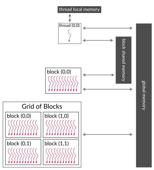
Figure 2. CUDA memory hierarchy. Every thread has access to global memory, only threads from a single
block have access to block shared memory and each thread has its own local memory.
(based on: http://docs.nvidia.com/cuda/cuda-c-programming-guide/index.html)
Implementation Plan
We know already fundamentals of CUDA programming. We can use that knowledge to prepare a simple feedforward neural network implementation and harness GPU power for this purpose. Let's say we want to be able to build a network shown in the figure 3. It is just linear layer followed by ReLU activation and one more linear layer followed by sigmoid activation.

Figure 3. The neural network we want to build using CUDA.
What do we need more? Ah yeah -- a cost function. Let's say we would like our network to solve binary classification problem, therefore we will use binary cross-entropy function. In order to implement a whole neural network we will need following classes:
- Matrix -- neural network is a fancy name but a great part of it boils down to tensor operations, in this case we just need a matrix (2nd order tensor)
- layers -- we need to implement forward and backward pass for every layer, i.e.
- SigmoidActivation
- ReLUActivation
- LinearLayer
- BCECost -- this will be a class responsible for computing binary cross-entropy cost and its derivative
- NeuralNetwork -- this one will keep everything together and will manage communication between all elements
Implementation
We will go through implementation of every class listed above, but to keep this post on track we will skip some implementation details. Complete working code along with unit tests is available at github. Let's start with Matrix class implementation.
Matrix Class
We need some data structure that will keep all the numbers and parameters -- a matrix. The important thing here is that we want a matrix to be available both on host memory (for CPU) and on device memory (for GPU). Most operations will be performed on device but we might need e.g. to initialize a matrix on host, just because it will be easier. Of course we could implement everything on device, but we want to keep it simple. Matrix class will manage memory allocation and make data transfer between host and device easier. On listing 4 you can see a Matrix class header.
Listing 4. Matrix class header.
class Matrix {
private:
    bool device_allocated;
    bool host_allocated;

    void allocateCudaMemory();
    void allocateHostMemory();

public:
    Shape shape;

    std::shared_ptr<float> data_device;
    std::shared_ptr<float> data_host;

    Matrix(size_t x_dim = 1, size_t y_dim = 1);
    Matrix(Shape shape);

    void allocateMemory();
    void allocateMemoryIfNotAllocated(Shape shape);

    void copyHostToDevice();
    void copyDeviceToHost();

    float& operator[](const int index);
    const float& operator[](const int index) const;
};
As you can see we are using smart pointers (std::shared_ptr) which will count references for us and deallocate memory when suitable (both on host and on device). In a while you will see how we will allocate device memory with smart pointer. The most important functions here are allocateMemory() (allocate memory on host and on device) and two functions for data transfer i.e. copyHostToDevice() and copyDeviceToHost(). A Shape is just a structure that keeps X and Y dimensions. allocateMemoryIfNotAllocated() function checks whether memory is already allocated and if not it will allocate memory for a matrix of a given shape. This will be useful when we won't know the matrix shape upfront. For convenience we overload subscript operator [] to have easy access to matrix values (from data_host). Let's look at functions performing memory allocation. In listings 5 and 6 you can see host memory allocation and device memory allocation using smart pointers.
Listing 5. Host memory allocation for a matrix.
void Matrix::allocateHostMemory() {
    if (!host_allocated) {
        data_host = std::shared_ptr<float>(new float[shape.x * shape.y],
                                           [&](float* ptr){ delete[] ptr; });
        host_allocated = true;
    }
}
As you can see in the listing 5 we have an ordinary memory allocation with new operator. We are passing pointer to an allocated memory to shared_ptr (1st argument). As smart pointer by default will call delete operator we need to pass also a second argument that will tell how to perform deallocation. We can put here a pointer to a function or, as we did here, enter a lambda expression with delete[] operator.
Listing 6. Device memory allocation for a matrix.
void Matrix::allocateCudaMemory() {
    if (!device_allocated) {
        float* device_memory = nullptr;
        cudaMalloc(&device_memory, shape.x * shape.y * sizeof(float));
        NNException::throwIfDeviceErrorsOccurred("Cannot allocate CUDA memory for Tensor3D.");
        data_device = std::shared_ptr<float>(device_memory,
                                             [&](float* ptr){ cudaFree(ptr); });
        device_allocated = true;
    }
}
In case of device memory allocation we need to perform analogous operations, but on device, i.e. for GPU. Firstly we allocate memory using cudaMalloc(...) function, then we pass a pointer to allocated memory space to shared_ptr. Again we are passing lambda expression as the second argument but this time we are deallocating device memory, so we need to use cudaFree(...) function instead of delete[] operator.
Memory allocation is the most important and usefull thing when it comes to Matrix class. allocateMemory() function just call two presented above functions. When it comes to copyHostToDevice() and copyDeviceToHost() functions they just call cudaMemcpy(...) function in suitable direction, i.e. from device to host or the other way around.
Layers Classes
Every class that will implement any neural network layer has to perform forward and backward propagation. What is more we want NeuralNetwork class to treat every layer the same way. We don't want to care about implementation details of layers classes, we just want to pass some data to every of them and get some results. All right, it sounds like we need polymorphism. We need an interface for all network layers -- you can see it in the listing 7.
Listing 7. An interface for neural network layers.
class NNLayer {
protected:
    std::string name;

public:
    virtual ~NNLayer() = 0;

    virtual Matrix& forward(Matrix& A) = 0;
    virtual Matrix& backprop(Matrix& dZ, float learning_rate) = 0;

    std::string getName() { return this->name; };
};
To sum this interface up, every layer is required to have forward(...) and backprop(...) functions. Each layer has also some name.
Sigmoid Layer
Both activation layers we are implementing are very simple. Sigmoid layer should compute sigmoid function for every matrix element in the forward pass. The sigmoid function is:
$$ \sigma(x) = \frac{e^x}{1 + e^x} $$
In the backward pass we need to use the chain rule which is foundation of backpropagation. We want to compute an error introduced by layer's input Z. We will denote this error as dZ. According to the chain rule:
$$ dZ = \frac{dJ}{d\sigma(x)} \frac{d\sigma(x)}{dx} = dA \cdot \sigma(x) \cdot \big(1 - \sigma(x)\big) $$
Where \(J\) is a cost function and \(\frac{dJ}{d\sigma(x)}\) is an error introduced by sigmoid layer -- we obtain it as backprop(...) function argument and we denote it as dA.
Below you can see how SigmoidActivation class header looks like.
Listing 8. SigmoidActivation class header.
class SigmoidActivation : public NNLayer {
private:
    Matrix A;

    Matrix Z;
    Matrix dZ;

public:
    SigmoidActivation(std::string name);
    ~SigmoidActivation();

    Matrix& forward(Matrix& Z);
    Matrix& backprop(Matrix& dA, float learning_rate = 0.01);
};
Note that we want to store layer's input Z as well as its output A. We want also to store output of backpropagation from this layer, this is denoted here by dZ (because we are calculating error introduced by layer's input Z).
I am using here following convention:
Zdenotes output of a linear layer,Adenotes output of activation layer. In general we can write operation performed by sigmoid function as \(A_n = \sigma(Z_n)\), where \(Z_n = W_nA_{n-1} + b_n\) is the output from linear layer.
We start by implementing CUDA kernels for our sigmoid layer. In the listing 9 you can see forward pass kernel.
Listing 9. SigmoidActivation forward pass CUDA kernel.
__device__ float sigmoid(float x) {
    return 1.0f / (1 + exp(-x));
}

__global__ void sigmoidActivationForward(float* Z, float* A,
                                         int Z_x_dim, int Z_y_dim) {
    int index = blockIdx.x * blockDim.x + threadIdx.x;

    if (index < Z_x_dim * Z_y_dim) {
        A[index] = sigmoid(Z[index]);
    }
}
The implementation is rather straightforward. We calculate index for current thread that is executing the kernel, then we check if this index is within matrix bounds and compute sigmoid activation. Every CUDA thread compute a single output. What might be new here is a function with __device__ keyword. This is a function that can be called only on device, e.g. by our kernel function, and is executed on device. On the other hand __global__ functions can be called from host and are executed on device.
Listing 10. SigmoidActivation backward pass CUDA kernel.
__global__ void sigmoidActivationBackprop(float* Z, float* dA, float* dZ,
                                          int Z_x_dim, int Z_y_dim) {
    int index = blockIdx.x * blockDim.x + threadIdx.x;

    if (index < Z_x_dim * Z_y_dim) {
        dZ[index] = dA[index] * sigmoid(Z[index]) * (1 - sigmoid(Z[index]));
    }
}
Backward pass logic is very similar to forward pass, the only difference is that this time we are implementing another equation. As we have kernels already implemented, we can call them in forward(...) and backprop(...) functions of SigmoidActivation class. Let's see how it is done.
Listing 11. Forward pass function in SigmoidActivation class.
Matrix& SigmoidActivation::forward(Matrix& Z) {
    this->Z = Z;
    A.allocateMemoryIfNotAllocated(Z.shape);

    dim3 block_size(256);
    dim3 num_of_blocks((Z.shape.y * Z.shape.x + block_size.x - 1) / block_size.x);

    sigmoidActivationForward<<<num_of_blocks, block_size>>>(Z.data_device.get(), A.data_device.get(),
                                                            Z.shape.x, Z.shape.y);
    NNException::throwIfDeviceErrorsOccurred("Cannot perform sigmoid forward propagation.");

    return A;
}
In forward pass we store Z input, because we will need it during backpropagation step. Then we make sure that output matrix A has allocated space and a proper shape. After that we compute number of blocks we need, so that every of them contains 256 threads. After computations we return result matrix A.
Listing 12. Backward pass function in SigmoidActivation class.
Matrix& SigmoidActivation::backprop(Matrix& dA, float learning_rate) {
    dZ.allocateMemoryIfNotAllocated(Z.shape);

    dim3 block_size(256);
    dim3 num_of_blocks((Z.shape.y * Z.shape.x + block_size.x - 1) / block_size.x);
    sigmoidActivationBackprop<<<num_of_blocks, block_size>>>(Z.data_device.get(), dA.data_device.get(),
                                                             dZ.data_device.get(),
                                                             Z.shape.x, Z.shape.y);
    NNException::throwIfDeviceErrorsOccurred("Cannot perform sigmoid back propagation");

    return dZ;
}
There is nothing extraordinary in backprop(...) function if we compare it with forward(...) function. We just make sure that dZ matrix, that is an output of this function, is correctly allocated. Next we define number of threads and blocks and call a kernel. This pattern repeats in every layer implementation, therefore I won't list these functions for further layers. The most interesting things for us are actually kernels and this is what we will analyse hereafter. If you are interested in all details, please check the github repository.
ReLU Layer
ReLUActivation class has almost the same header as SigmoidActivation class, so we skip it. The main difference here is equation defining ReLU function:
$$ ReLU(x) = \begin{cases}
x & \text{ for } x > 0 \\
0 & \text { otherwise}
\end{cases} = max(0, x)$$
Note that derivative of ReLU function is 1 when x > 0 and 0 otherwise. Therefore for backpropagation, using the chain rule, we obtain following formula to implement:
$$ dZ = \frac{dJ}{dReLU(x)} \frac{dReLU(x)}{dx} = \begin{cases}
dA & \text{ for } x > 0 \\
0 & \text { otherwise}
\end{cases} $$
In the listing 13 you can find implementation of the forward pass kernel.
Listing 13. ReLUActivation forward pass CUDA kernel.
__global__ void reluActivationForward(float* Z, float* A,
                                      int Z_x_dim, int Z_y_dim) {
    int index = blockIdx.x * blockDim.x + threadIdx.x;

    if (index < Z_x_dim * Z_y_dim) {
        A[index] = fmaxf(Z[index], 0);
    }
}
As we already know equations, implementing CUDA kernels is quite simple and in its logic very similar to sigmoid layer kernels. Within CUDA kernels we can use number of math built-in functions, one of them is fmaxf function. More on built-in functions you can find in CUDA Math API Documentation. Now it's time for backward pass implementation.
Listing 14. ReLUActivation backward pass CUDA kernel.
__global__ void reluActivationBackprop(float* Z, float* dA, float* dZ,
                                       int Z_x_dim, int Z_y_dim) {
    int index = blockIdx.x * blockDim.x + threadIdx.x;

    if (index < Z_x_dim * Z_y_dim) {
        if (Z[index] > 0) {
            dZ[index] = dA[index];
        }
        else {
            dZ[index] = 0;
        }
    }
}
Again, we just implement equation presented above. There is one thing worth to notice in this place. We had to use if statement here in order to check whether Z input was greater or lower than 0. This cause that some threads will execute different set of instructions than other threads. This hugely affects the kernel performance and we should in general avoid if statements in our kernels as much as possible. On the other hand the first if that checks matrix bounds is not so adverse, because most threads execute the same code anyway (most threads will have index within matrix bound). This is called thread divergence and I will write more about it in the part 2 of this post.
Linear Layer
LinearLayer class is more interesting than classes of activation functions because it has parameters W and b, so a bit more happens here. In particular we need to implement gradient descent to update these parameters during back propagation. As for previous layers we will start with equations. Linear layer in a forward pass should implement following equation:
$$ Z = WA + b $$
Where \(W\) is weights matrix, \(b\) is bias vector and \(A\) is input to this layer. Note that this time we are computing \(Z\), not \(A\) as in case of activation layers. Furthermore we need three derivatives this time. One to find out what error was introduced by input \(A\), and this one should be passed to preceding layer during back propagation. We need also to know what error was introduced by \(W\) and \(b\) to be able to update these parameters accordingly using gradient descent.
$$ dA = \frac{dJ}{dZ} \frac{dZ}{dA} = W^T \cdot dZ $$
$$ dW = \frac{dJ}{dZ} \frac{dZ}{dW} = \frac{1}{m} \cdot dZ \cdot A^T $$
$$ db = \frac{dJ}{dZ} \frac{dZ}{db} = \frac{1}{m} \sum_{i=0}^m dZ^{(i)} $$
Where \(dZ^{(i)}\) is \(i\)'th column of \(dZ\) (\(i\)'th input in a batch) and \(m\) is size of a batch. Below you can see how the header of LinearLayer class looks like.
Listing 15. LinearLayer class header.
class LinearLayer : public NNLayer {
private:
    const float weights_init_threshold = 0.01;

    Matrix W;
    Matrix b;

    Matrix Z;
    Matrix A;
    Matrix dA;

    void initializeBiasWithZeros();
    void initializeWeightsRandomly();

    void computeAndStoreBackpropError(Matrix& dZ);
    void computeAndStoreLayerOutput(Matrix& A);
    void updateWeights(Matrix& dZ, float learning_rate);
    void updateBias(Matrix& dZ, float learning_rate);

public:
    LinearLayer(std::string name, Shape W_shape);
    ~LinearLayer();

    Matrix& forward(Matrix& A);
    Matrix& backprop(Matrix& dZ, float learning_rate = 0.01);

    int getXDim() const;
    int getYDim() const;

    Matrix getWeightsMatrix() const;
    Matrix getBiasVector() const;
};
As a quick overview let's skim over functions of this class. Of course we have forward(...) and backprop(...) functions here and additionally we have some set of getters. We have two initialization methods here, i.e. for bias initialization and for weights initialization. We will initialize bias vector all with zeros and we will initialize weights matrix with values from normal distribution with 0 mean and standard deviation equal to 1. These will be additionally multiplied by weights_init_threshold value. If you are interested in mentioned initialization methods you can find details in the github repository. I guess that computeAndStore and update functions are self-explanatory. These are just helper functions that will call relevant kernel and these are used in forward(...) and backprop(...) functions. Let's go straight to the most interesting part that are CUDA kernels.
This time we don't have to compute a function value for every matrix element independently as in case of activation functions. Now we need to compute matrices product. We should avoid synchronization of threads if it is possible, bacause it slows down our kernel. In order to omit the synchronization two threads cannot write to the same localization because otherwise we will have race conditions. On the other hand our threads can read from the same location simultaneously, i.e. values from multiplied matrices, because we know that these won't change during computations. We can do this easily by asking every thread to calculate a single element of an output matrix. You can see it in the figure 4. Every single thread will compute a single pink dot. Every pink dot is a dot product of row from matrix A and a column from matrix B.
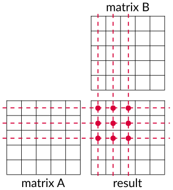
Figure 4. Matrix-matrix multiplication. We are computing pink dots and each dot is a dot product of row lying
on dashed line and column lying on dotted line.
In the listing 16 you can find how forward propagation is implemented as a CUDA kernel.
Listing 16. LinearLayer forward pass CUDA kernel.
__global__ void linearLayerForward( float* W, float* A, float* Z, float* b,
                                    int W_x_dim, int W_y_dim,
                                    int A_x_dim, int A_y_dim) {
    int row = blockIdx.y * blockDim.y + threadIdx.y;
    int col = blockIdx.x * blockDim.x + threadIdx.x;

    int Z_x_dim = A_x_dim;
    int Z_y_dim = W_y_dim;

    float Z_value = 0;

    if (row < Z_y_dim && col < Z_x_dim) {
        for (int i = 0; i < W_x_dim; i++) {
            Z_value += W[row * W_x_dim + i] * A[i * A_x_dim + col];
        }
        Z[row * Z_x_dim + col] = Z_value + b[row];
    }
}
Until now, we were creating 1D threads grid but here we create 2D threads grid. It makes things a bit easier, because by Y thread's index we can get a row of the result matrix and by X thread's index we get a column of the result matrix. Then we simply multiply each row element of matrix W with each column element of matrix A. Finally we add a bias to our result. That's it. We computed output of a linear layer forward pass, i.e. Z matrix. Now we need to implement a whole backpropagation step. First of all we need to compute dA that will be passed to preceding layer.
Listing 17. LinearLayer backward pass CUDA kernel (computing `dA`).
__global__ void linearLayerBackprop(float* W, float* dZ, float *dA,
                                    int W_x_dim, int W_y_dim,
                                    int dZ_x_dim, int dZ_y_dim) {
    int col = blockIdx.x * blockDim.x + threadIdx.x;
    int row = blockIdx.y * blockDim.y + threadIdx.y;

    // W is treated as transposed
    int dA_x_dim = dZ_x_dim;
    int dA_y_dim = W_x_dim;

    float dA_value = 0.0f;

    if (row < dA_y_dim && col < dA_x_dim) {
        for (int i = 0; i < W_y_dim; i++) {
            dA_value += W[i * W_x_dim + row] * dZ[i * dZ_x_dim + col];
        }
        dA[row * dA_x_dim + col] = dA_value;
    }
}
This kernel is quite similar to this for forward pass. The only difference is that we need W matrix to be transposed. Instead of making separate kernel for transposition we can simply multiply each W column by dZ columns. It will be equivalent of computing transpose(W)*dZ. Next step is to update linear layer's weights accordingly to dZ which is presented in the listing 18.
Listing 18. LinearLayer weights update CUDA kernel (gradient descent).
__global__ void linearLayerUpdateWeights(  float* dZ, float* A, float* W,
                                           int dZ_x_dim, int dZ_y_dim,
                                           int A_x_dim, int A_y_dim,
                                           float learning_rate) {
    int col = blockIdx.x * blockDim.x + threadIdx.x;
    int row = blockIdx.y * blockDim.y + threadIdx.y;

    // A is treated as transposed
    int W_x_dim = A_y_dim;
    int W_y_dim = dZ_y_dim;

    float dW_value = 0.0f;

    if (row < W_y_dim && col < W_x_dim) {
        for (int i = 0; i < dZ_x_dim; i++) {
            dW_value += dZ[row * dZ_x_dim + i] * A[col * A_x_dim + i];
        }
        W[row * W_x_dim + col] = W[row * W_x_dim + col] - learning_rate * (dW_value / A_x_dim);
    }
}
We apply similar trick here to pretend that A matrix is transposed. The final step in this kernel is updating weights matrix. We are using the simplest form of gradient descent here and just subtract gradient value multiplied by learning rate from current weights matrix. The last step during backpropagation in our linear layer is performing bias vector update.
Listing 19. LinearLayer bias update CUDA kernel (gradient descent).
__global__ void linearLayerUpdateBias(  float* dZ, float* b,
                                        int dZ_x_dim, int dZ_y_dim,
                                        int b_x_dim,
                                        float learning_rate) {
    int index = blockIdx.x * blockDim.x + threadIdx.x;

    if (index < dZ_x_dim * dZ_y_dim) {
        int dZ_x = index % dZ_x_dim;
        int dZ_y = index / dZ_x_dim;
        atomicAdd(&b[dZ_y], - learning_rate * (dZ[dZ_y * dZ_x_dim + dZ_x] / dZ_x_dim));
    }
}
Bias update kernel is very simple and we simply apply gradient descent rule. What is iteresting in this kernel is usage of atomicAdd(...) function. When we implement bias update this way, multiple threads will write to the same memory location, i.e. bias vector elements. We have to make sure that we won't have race conditions here, therefore we call atomic operation that guarantee that another thread will have access to memory location when current thread complete his addition operation. Nevertheless, using atomic operations in CUDA kernels is undesirable because it harms kernel performance. Instead of quickly performing a lot of operations, some threads need to wait for their turn. Of course, sometimes we just have to use atomic operations and CUDA provides some set of such.
All right. Implementation of all neural network layers is ready. We still need a cost function.
Binary Cross-Entropy
We have decided to use binary cross-entropy cost function, so what do we need exactly? Well, just a function that computes a cost and a function that returns gradient accordingly to network predictions and our target values. Binary cross-entropy is defined with following equation:
$$ BCE = - \frac{1}{m} \sum_{i=0}^m (y\log(\hat{y}) + (1 - y)\log(1 - \hat{y})) $$
And by calculating its derivative we compute gradient as:
$$ \bigtriangledown BCE = - (\frac{y}{\hat{y}} - \frac{1 - y}{1 - \hat{y}}) $$
Where by \(\hat{y}\) we denote predicted values and by \(y\) the ground truth values. The header of BCECost class is straightforward.
Listing 20. BCECost class header.
class BCECost {
public:
    float cost(Matrix predictions, Matrix target);
    Matrix dCost(Matrix predictions, Matrix target, Matrix dY);
};
Nothing extraordinary happens in BCE cost calculation kernel. Note that we use again built-in math function, this time logf.
Listing 21. BCECost --- cost calculation CUDA kernel.
__global__ void binaryCrossEntropyCost(float* predictions, float* target,
                                       int size, float* cost) {
    int index = blockIdx.x * blockDim.x + threadIdx.x;

    if (index < size) {
        float partial_cost = target[index] * logf(predictions[index])
                + (1.0f - target[index]) * logf(1.0f - predictions[index]);
        atomicAdd(cost, - partial_cost / size);
    }
}
And below is gradient computation kernel.
Listing 22. BCECost --- cost function gradient calculation CUDA kernel.
__global__ void dBinaryCrossEntropyCost(float* predictions, float* target, float* dY,
                                        int size) {
    int index = blockIdx.x * blockDim.x + threadIdx.x;

    if (index < size) {
        dY[index] = -1.0 * ( target[index]/predictions[index] - (1 - target[index])/(1 - predictions[index]) );
    }
}
So far we have implemented all fundamental building blocks of our neural network. We just need one more class -- NeuralNetwork, that will keep them all together.
NeuralNetwork Class
This class is responsible for managing all network components and also to communicate layers with each other during forward and during backward passes. Let's look at its header declaration.
Listing 23. NeuralNetwork class header.
class NeuralNetwork {
private:
    std::vector<NNLayer*> layers;
    BCECost bce_cost;

    Matrix Y;
    Matrix dY;
    float learning_rate;

public:
    NeuralNetwork(float learning_rate = 0.01);
    ~NeuralNetwork();

    Matrix forward(Matrix X);
    void backprop(Matrix predictions, Matrix target);

    void addLayer(NNLayer *layer);
    std::vector<NNLayer*> getLayers() const;
};
Our NeuralNetwork class keeps all layers in layers vector. We can add new layers using addLayer(...) function. The class holds also cost function object. We could probably make this more generic to allow user to put his own cost function, but let's leave it that way for now. The most important functions here are forward(...) and backprop(...). These function are just passing output from one layer to the next one (forward pass), or to the previous one in case of back propagation. In the listing 23 you can find code of the forward(...) function.
Listing 24. NeuralNetwork --- forward pass function.
Matrix NeuralNetwork::forward(Matrix X) {
    Matrix Z = X;

    for (auto layer : layers) {
        Z = layer->forward(Z);
    }

    Y = Z;
    return Y;
}
As you can see, all we do here is to iterate over every layer and pass output from one layer to another. Of course, to the first layer in the vector we pass network input X. The backprop(...) function is very similar, but we have to use reversed iterator to go through the layers vector from the last layer to the first one.
Listing 25. NeuralNetwork --- backward pass function.
void NeuralNetwork::backprop(Matrix predictions, Matrix target) {
    dY.allocateMemoryIfNotAllocated(predictions.shape);
    Matrix error = bce_cost.dCost(predictions, target, dY);

    for (auto it = this->layers.rbegin(); it != this->layers.rend(); it++) {
        error = (*it)->backprop(error, learning_rate);
    }

    cudaDeviceSynchronize();
}
Back propagation function takes as its arguments predicted and target values, computes gradient of BCE cost and then passes errors between all network layers calling their backprop(...) functions. A new thing here is cudaDeviceSynchronize() call. This function waits untill all CUDA threads end its job. It is similar to join() function when we are working with traditional threads. We need this function because we want to get cost value from host code during training time. We have to be certain that all computations are over, otherwise we can obtain some pseudorandom values.
Training
We have implemented everything we need to build neural network based on linear layers, ReLU and sigmoid activations and binary cross-entropy cost. Let's create a neural network that was described at the beginning and train it to predict some values. I created CoordinatesDataset class to check whether our network is able to learn something. It just draws random coordinates in 2D space. We want to predict whether a point lies within 1st or 3rd quadrant or whether it lies within 2nd or 4th quadrant.
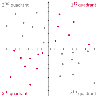
Figure 5. Coordinates dataset. Pink dots belong to one class and gray ones to another.
It is time to add some layers to our network and try to train it so it will predict to which class a given point in 2D space belongs.
Listing 26. Building and training planned neural network.
int main() {

    srand( time(NULL) );

    CoordinatesDataset dataset(100, 21);
    BCECost bce_cost;

    NeuralNetwork nn;
    nn.addLayer(new LinearLayer("linear_1", Shape(2, 30)));
    nn.addLayer(new ReLUActivation("relu_1"));
    nn.addLayer(new LinearLayer("linear_2", Shape(30, 1)));
    nn.addLayer(new SigmoidActivation("sigmoid_output"));

    // network training
    Matrix Y;
    for (int epoch = 0; epoch < 1001; epoch++) {
        float cost = 0.0;

        for (int batch = 0; batch < dataset.getNumOfBatches() - 1; batch++) {
            Y = nn.forward(dataset.getBatches().at(batch));
            nn.backprop(Y, dataset.getTargets().at(batch));
            cost += bce_cost.cost(Y, dataset.getTargets().at(batch));
        }

        if (epoch % 100 == 0) {
            std::cout   << "Epoch: " << epoch
                        << ", Cost: " << cost / dataset.getNumOfBatches()
                        << std::endl;
        }
    }

    // compute accuracy
    Y = nn.forward(dataset.getBatches().at(dataset.getNumOfBatches() - 1));
    Y.copyDeviceToHost();

    float accuracy = computeAccuracy(
            Y, dataset.getTargets().at(dataset.getNumOfBatches() - 1));
    std::cout   << "Accuracy: " << accuracy << std::endl;

    return 0;
}
At the beginning we create a dataset with 21 batches, every one containing 100 data points. We will use 20 batches for training and the last one as our test set to check the final accuracy score. Then we populate our neural network with some layers. First layer takes batch of points, so we have 2 inputs here and we would like to have 30 neurons in the hidden layer. Then we add ReLU activation and define new linear layer with 30 neurons that will output just a single value that will be activated with sigmoid function. The next part is a training. We are going to train the network over 1000 epochs and print the cost after every 100 epochs. After training we can check the accuracy score of our neural network. computeAccuracy(...) function just counts number of correctly predicted values and divides it by the size of output vector. You can find the output in listing 25.
Listing 27. Neural network training output.
Epoch: 0, Cost: 0.660046
Epoch: 100, Cost: 0.658017
Epoch: 200, Cost: 0.657598
Epoch: 300, Cost: 0.656288
Epoch: 400, Cost: 0.652261
Epoch: 500, Cost: 0.640935
Epoch: 600, Cost: 0.615166
Epoch: 700, Cost: 0.573332
Epoch: 800, Cost: 0.518711
Epoch: 900, Cost: 0.43961
Epoch: 1000, Cost: 0.343429
Accuracy: 0.93
As you can see the neural network converges over number of epochs. The convergence is a little bit slow which is probably a result of using simple gradient descent. After 1000 epochs the network scores 93% on accuracy. With such simple dataset we can easily make it 100% with more epochs. Finally it seems that our CUDA implementation of neural network is working correctly.
Conclusion
In this a little bit lenghty post we have implemented simple neural network using CUDA technology and performed the crucial operations on GPU processor. GPU is great for massively parallel operations such as matrix operations. However, originally GPUs were not designed for general-purpose computations including neural networks implementation. This is one of reasons why hardware companies are still working on much more suitable processor architectures to get as high performance as possible on such applications, though it's a topic for another post.
An important thing is that writing CUDA kernels is not as easy as it might seem at first glance. We have to be cautious about different conditions and restrictions to make computations correct but also to not harm kernels performance. What you have seen in this post is a very simple implementation and it can be improved. This is definitely not the implementation you would find if you take a look at popular deep learning libraries repositories. Nevertheless, I hope it shows that there is quite a lot going on under the hood of python deep learning libraries. I am going to write a second part of this post, where I will focus more on the performance issues and possible improvements of this implementation.
Further Reading
GitHub Repository -- Here you can find complete code for the project presented in this post along with unit tests.
An Even Easier Introduction to CUDA -- An excelent introduction to CUDA. It uses unified memory instead of manual transfer of data between host and device.
Unified Memory in CUDA 6 -- More information on Unified Memory introduced in CUDA 6.
CUDA Thread Execution Model -- An extensive information on CUDA thread execution model. You can find here more about thread synchronization, scheduling and divergence.
CUDA Toolkit Documentation -- Everything you might need when working with CUDA.
Also published on Medium.